Effect sizes are a quantitative measure of the magnitude (size) of a phenomenon. Unlike p-values, which tell you if an effect exists, effect sizes tell you how large that effect is. They are very important for understanding the practical significance of research findings.
p-values (e.g., p < 0.05) indicate whether an observed difference or relationship is likely to have occurred by chance. Effect sizes measure the strength of these differences or relationships.
Just because something is statistically significant doesn’t make it important.
They help us to understand the real-world importance of our results, to compare research findings across studies with different scales or sample sizes, and to make informed decisions about the practical implications of our research.
40.2 Using Cohen’s D
Cohen’s D is used to measure the difference between two groups’ means in relation to their standard deviation, quantifying the size of the effect.
It’s particularly useful in comparing the effects of treatments or interventions across different studies or experiments.
A Cohen’s D value closer to 0 suggests a small effect size, meaning there’s little to no practical difference between the two groups.
Values further away from 0 (either positive or negative) indicate a larger effect size, suggesting a more significant difference between the group means.
This measure helps us understand the magnitude of an effect beyond just noting its statistical significance, helping us evaluate how meaningful the differences are in practical terms.
Show code for dataset generation
rm(list=ls())# Load packageslibrary(effsize)library(psych)# Function to generate datagenerate_data <-function(n =100, mean1 =50, sd1 =10, mean2 =60, sd2 =10) {set.seed(123) # For reproducibility# Generate data for two groups group1 <-rnorm(n, mean1, sd1) group2 <-rnorm(n, mean2, sd2)# Combine into a data frame data <-data.frame(score =c(group1, group2),group =factor(c(rep("Group1", n), rep("Group2", n))) )return(data)}# Generate the datasetdata <-generate_data()## Dataset Two# Set seed for reproducibilityset.seed(123)# Parametersn <-100# Number of observations per groupmean_group1 <-50# Mean of group 1mean_group2 <-52# Mean of group 2 (slightly higher to ensure a small effect size)sd_both <-6# Standard deviation for both groups# Generate datagroup1 <-rnorm(n, mean_group1, sd_both)group2 <-rnorm(n, mean_group2, sd_both)# Combine into a data frame data2 <-data.frame(score =c(group1, group2),group =factor(c(rep("Group1", n), rep("Group2", n))) )
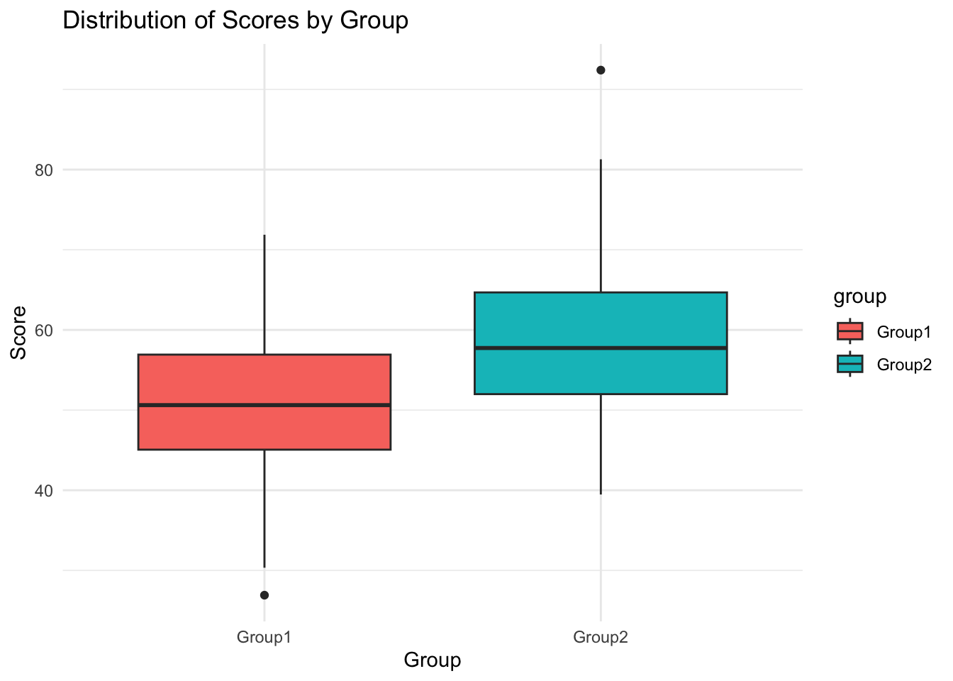
#----------------# Visualise distributionlibrary(ggplot2)ggplot(data, aes(x = group, y = score, fill = group)) +geom_boxplot() +theme_minimal() +labs(title ="Distribution of Scores by Group", x ="Group", y ="Score")
#----------------# Look for between-group differences using t-testt.test(score ~ group, data = data, alternative ="two.sided", var.equal =FALSE, conf.level =0.95)
    Welch Two Sample t-test

data:  score by group
t = -6.0315, df = 197.35, p-value = 7.88e-09
alternative hypothesis: true difference in means between group Group1 and group Group2 is not equal to 0
95 percent confidence interval:
 -10.642862  -5.398084
sample estimates:
mean in group Group1 mean in group Group2
            50.90406             58.92453
#----------------# Calculate Cohen's D# using effsized <-cohen.d(data$score,data$group)print(d)
Call: cohen.d(x = data$score, group = data$group)
Cohen d statistic of difference between two means
     lower effect upper
[1,]  0.57   0.86  1.15

Multivariate (Mahalanobis) distance between groups
[1] 0.86
r equivalent of difference between two means
data
0.39
Magnitude of the Effect
The absolute value of Cohen’s D helps you assess the magnitude of the effect:
Small effect size: d=0.2
Medium effect size: d=0.5
Large effect size: d>=0.8
What is Mahalanobis Distance?
Mahalanobis distance is used to determine the distance between a point and a distribution. It’s particularly useful for assessing how many standard deviations away a point is from the mean of a distribution, taking into account the covariance among variables.
40.3 Using Pearson’s R
Pearson’s correlation coefficient (‘Pearson’s R’) is a measure of the strength and direction of a linear relationship between two continuous variables.
It ranges from -1 to 1: - -1 indicates a perfect negative linear relationship - 1 indicates a perfect positive linear relationship - 0 indicates no linear relationship.
# Sample data set.seed(123) # For reproducibilityx <-rnorm(100, mean =50, sd =10) # Variable 1y <- x *1.5+rnorm(100, mean =0, sd =5) # Variable 2, correlated with x# Calculate Pearson's correlationpearson_r <-cor(x, y, method ="pearson")cat("\nPearson R Result:\n")
Pearson R Result:
print(pearson_r)
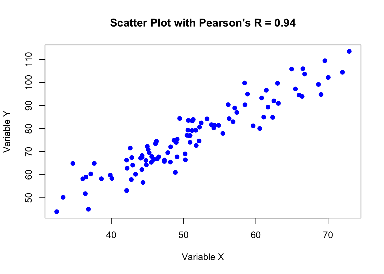
[1] 0.937795
# Scatter plot of x and yplot(x, y, main =paste("Scatter Plot with Pearson's R =", round(pearson_r, 2)), xlab ="Variable X", ylab ="Variable Y", pch =19, col ="blue")
# Test for significancecor_test_result <-cor.test(x, y, method ="pearson")cat("\nCor Test Result:\n")
Cor Test Result:
print(cor_test_result)
    Pearson's product-moment correlation

data:  x and y
t = 26.74, df = 98, p-value < 2.2e-16
alternative hypothesis: true correlation is not equal to 0
95 percent confidence interval:
 0.9087728 0.9577885
sample estimates:
     cor
0.937795
40.4 Using Odds Ratios
Odds ratios (OR) are used to show the relationship between two binary (yes/no) variables, commonly used in studies to compare how likely an event is to happen in one group versus another.
If the OR is greater than 1, it means the event is more likely in the first group.
If it’s less than 1, the event is less likely in the first group.
An OR of 1 means there’s no difference between the groups.
This helps us understand the real-world impact of treatments or risk factors on outcomes like disease presence, making it easier to decide on health policies or treatments.
Essentially, ORs help to measure and communicate the effectiveness or risk associated with a particular condition or treatment.
Let’s simulate a dataset for a hypothetical medical study comparing the effect of a treatment versus a placebo on a binary outcome (e.g., disease: present or absent).
Show code for dataset generation
# Set seed for reproducibilityset.seed(123)# Generate synthetic datan <-1000# Number of observations# Randomly assign treatment or control groupgroup <-sample(c("Treatment", "Control"), size = n, replace =TRUE)# Simulate outcome based on group# Assuming treatment group has lower odds of diseaseoutcome <-ifelse(group =="Treatment",rbinom(n, 1, 0.3), # 30% probability of disease in treatment grouprbinom(n, 1, 0.5)) # 50% probability of disease in control group# Create data framedata3 <-data.frame(group, outcome)
To calculate the odds ratio, we first need to create a 2x2 contingency table and then apply the appropriate statistical test (Fisher):
# Create a 2x2 tabletable_data <-table(data3$group, data3$outcome)colnames(table_data) <-c("No Disease", "Disease")# Calculate Odds Ratio and its 95% Confidence Interval using fisher.testor_test <-fisher.test(table_data)# Extract the Odds Ratio and its confidence intervalodds_ratio <- or_test$estimateconf_interval <- or_test$conf.int# Print the resultscat("Odds Ratio:", odds_ratio, "\n")
An OR < 1 suggests that the treatment group has lower odds of disease compared to the control group, indicating a protective effect of the treatment.
An OR > 1 would suggest higher odds of disease in the treatment group, indicating a risk factor.
An OR = 1 means there is no difference in odds between the two groups.
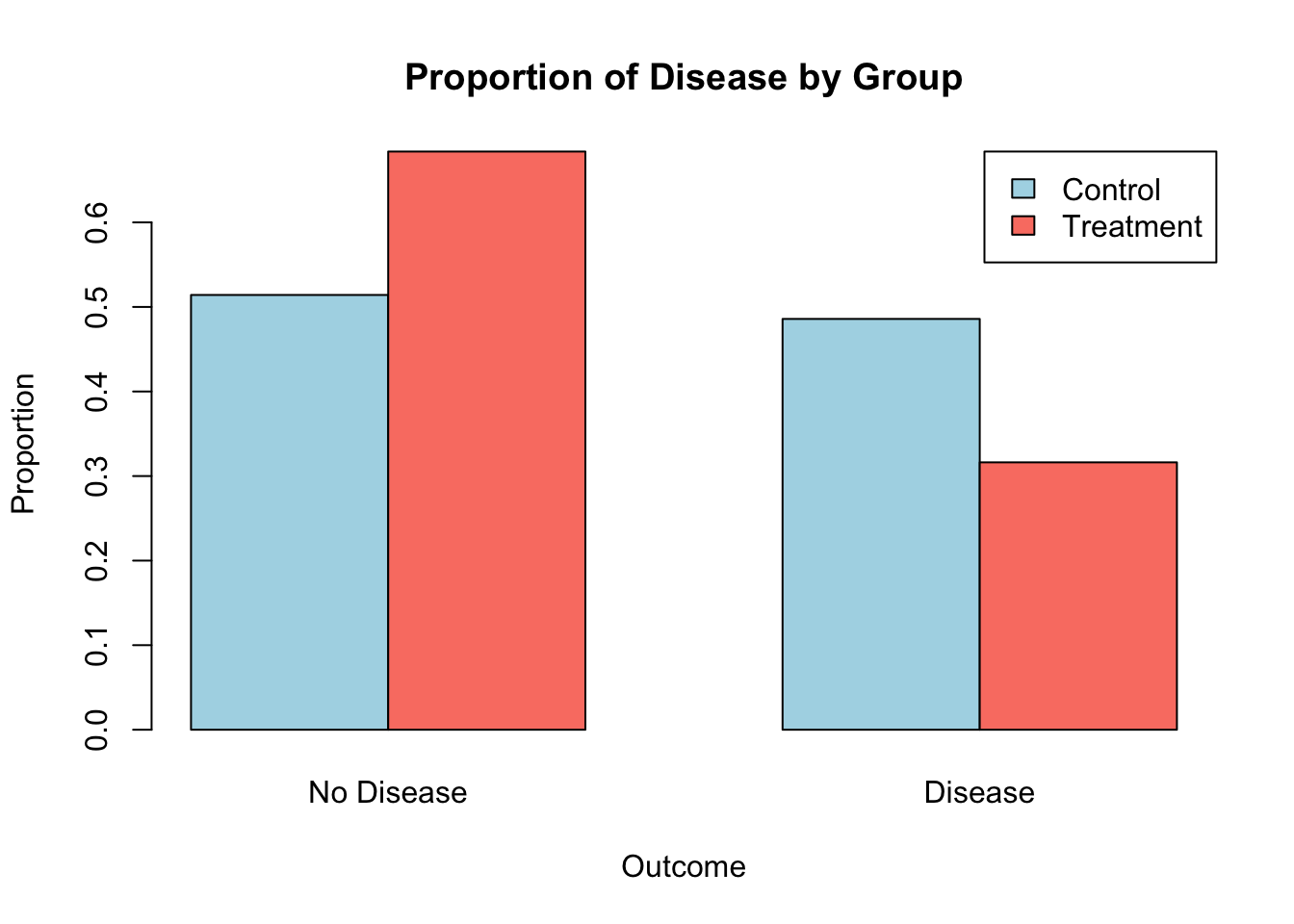
A simple way to visualise this is to create a bar plot showing the proportion of disease presence versus absence in each group.
# Calculate proportionsprop_table <-prop.table(table_data, 1) # Proportions by row# Bar plotbarplot(prop_table, beside =TRUE, col =c("lightblue", "salmon"),legend =TRUE, args.legend =list(x ="topright"),names.arg =c("No Disease", "Disease"),xlab ="Outcome", ylab ="Proportion",main ="Proportion of Disease by Group")
40.5 What if I have more than two groups or variables?
The ideas introduced above cover situations where we have two groups, or two variables.
The principles can be extended to (for example) techniques like ANOVA (Analysis of Variance) for comparing means across several groups, or by using multiple regression analysis, which can show how various factors affect an outcome together.
It’s worth exploring this further if you are dealing with data that is more complex, as effect sizes are generally mandatory in terms of reporting within peer-reviewed journal articles/conference papers.